Note
Get this example as a Jupyter Notebook ipynb
Using dask
dask is a Python package built upon the scientific stack to enable scalling of Python through interactive sessions to multi-core and multi-node.
Of particular relevance to SEGY-SAK is that xrray.Dataset loads naturally into dask.
Imports and Setup
Here we import the plotting tools, numpy and setup the dask.Client which will auto start a localcluster. Printing the client returns details about the dashboard link and resources.
[2]:
import numpy as np
from segysak import open_seisnc, segy

import matplotlib.pyplot as plt

%matplotlib inline
[3]:
from dask.distributed import Client

client = Client()
client
[3]:
Client
Client-5e95eb51-898c-11ec-89a5-ddf70e9c7bbb
| Connection method: Cluster object | Cluster type: distributed.LocalCluster |
| Dashboard: http://127.0.0.1:8787/status |
Cluster Info
LocalCluster
bfcd92e7
| Dashboard: http://127.0.0.1:8787/status | Workers: 2 |
| Total threads: 2 | Total memory: 6.78 GiB |
| Status: running | Using processes: True |
Scheduler Info
Scheduler
Scheduler-0fadbcee-eea8-4ab7-ac82-da9dc1f36ea7
| Comm: tcp://127.0.0.1:34223 | Workers: 2 |
| Dashboard: http://127.0.0.1:8787/status | Total threads: 2 |
| Started: Just now | Total memory: 6.78 GiB |
Workers
Worker: 0
| Comm: tcp://127.0.0.1:36775 | Total threads: 1 |
| Dashboard: http://127.0.0.1:41925/status | Memory: 3.39 GiB |
| Nanny: tcp://127.0.0.1:43011 | |
| Local directory: /home/runner/work/segysak/segysak/examples/dask-worker-space/worker-4mr7fea2 | |
Worker: 1
| Comm: tcp://127.0.0.1:44675 | Total threads: 1 |
| Dashboard: http://127.0.0.1:34059/status | Memory: 3.39 GiB |
| Nanny: tcp://127.0.0.1:44105 | |
| Local directory: /home/runner/work/segysak/segysak/examples/dask-worker-space/worker-7e3j_v01 | |
We can also scale the cluster to be a bit smaller.
[4]:
client.cluster.scale(2, memory="0.5gb")
client
[4]:
Client
Client-5e95eb51-898c-11ec-89a5-ddf70e9c7bbb
| Connection method: Cluster object | Cluster type: distributed.LocalCluster |
| Dashboard: http://127.0.0.1:8787/status |
Cluster Info
LocalCluster
bfcd92e7
| Dashboard: http://127.0.0.1:8787/status | Workers: 2 |
| Total threads: 2 | Total memory: 6.78 GiB |
| Status: running | Using processes: True |
Scheduler Info
Scheduler
Scheduler-0fadbcee-eea8-4ab7-ac82-da9dc1f36ea7
| Comm: tcp://127.0.0.1:34223 | Workers: 2 |
| Dashboard: http://127.0.0.1:8787/status | Total threads: 2 |
| Started: Just now | Total memory: 6.78 GiB |
Workers
Worker: 0
| Comm: tcp://127.0.0.1:36775 | Total threads: 1 |
| Dashboard: http://127.0.0.1:41925/status | Memory: 3.39 GiB |
| Nanny: tcp://127.0.0.1:43011 | |
| Local directory: /home/runner/work/segysak/segysak/examples/dask-worker-space/worker-4mr7fea2 | |
Worker: 1
| Comm: tcp://127.0.0.1:44675 | Total threads: 1 |
| Dashboard: http://127.0.0.1:34059/status | Memory: 3.39 GiB |
| Nanny: tcp://127.0.0.1:44105 | |
| Local directory: /home/runner/work/segysak/segysak/examples/dask-worker-space/worker-7e3j_v01 | |
Lazy loading from SEISNC using chunking
If your data is in SEG-Y to use dask it must be converted to SEISNC. If you do this with the CLI it only need happen once.
[5]:
segy_file = "data/volve10r12-full-twt-sub3d.sgy"
seisnc_file = "data/volve10r12-full-twt-sub3d.seisnc"
segy.segy_converter(
    segy_file, seisnc_file, iline=189, xline=193, cdpx=181, cdpy=185, silent=True
)
header_loaded
is_3d
Fast direction is INLINE_3D
By specifying the chunks argument to the open_seisnc command we can ask dask to fetch the data in chunks of size n. In this example the iline dimension will be chunked in groups of 100. The valid arguments to chunks depends on the dataset but any dimension can be used.
Even though the seis of the dataset is 2.14GB it hasn’t yet been loaded into memory, not will dask load it entirely unless the operation demands it.
[6]:
seisnc = open_seisnc("data/volve10r12-full-twt-sub3d.seisnc", chunks={"iline": 100})
seisnc.seis.humanbytes
[6]:
'40.05 MB'
Lets see what our dataset looks like. See that the variables are dask.array. This means they are references to the on disk data. The dimensions must be loaded so dask knows how to manage your dataset.
[7]:
seisnc
[7]:
<xarray.Dataset>
Dimensions:  (iline: 61, xline: 202, twt: 850)
Coordinates:
    cdp_x    (iline, xline) float32 dask.array<chunksize=(61, 202), meta=np.ndarray>
    cdp_y    (iline, xline) float32 dask.array<chunksize=(61, 202), meta=np.ndarray>
  * iline    (iline) uint16 10090 10091 10092 10093 ... 10147 10148 10149 10150
  * twt      (twt) float64 4.0 8.0 12.0 16.0 ... 3.392e+03 3.396e+03 3.4e+03
  * xline    (xline) uint16 2150 2151 2152 2153 2154 ... 2348 2349 2350 2351
Data variables:
    data     (iline, xline, twt) float32 dask.array<chunksize=(61, 202, 850), meta=np.ndarray>
Attributes: (12/13)
    coord_scalar:        -100.0
    measurement_system:  m
    percentiles:         [-6.59506019e+00 -6.11493624e+00 -1.50399996e+00 -3....
    sample_rate:         4.0
    source_file:         volve10r12-full-twt-sub3d.sgy
    text:                C 1 SEGY OUTPUT FROM Petrel 2017.2 Saturday, June 06...
    ...                  ...
    d3_domain:           None
    epsg:                None
    corner_points:       None
    corner_points_xy:    None
    srd:                 None
datatype: NoneOperations on SEISNC using dask
In this simple example we calculate the mean, of the entire cube. If you check the dashboard (when running this example yourself). You can see the task graph and task stream execution.
[8]:
mean = seisnc.data.mean()
mean
[8]:
<xarray.DataArray 'data' ()>
dask.array<mean_agg-aggregate, shape=(), dtype=float32, chunksize=(), chunktype=numpy.ndarray>
Whoa-oh, the mean is what? Yeah, dask won’t calculate anything until you ask it to. This means you can string computations together into a task graph for lazy evaluation. To get the mean try this
[9]:
mean.compute().values
[9]:
array(-7.317369e-05, dtype=float32)
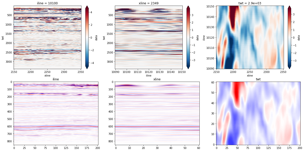
Plotting with dask
The lazy loading of data means we can plot what we want using xarray style slicing and dask will fetch only the data we need.
[10]:
fig, axs = plt.subplots(nrows=2, ncols=3, figsize=(20, 10))

iline = seisnc.sel(iline=10100).transpose("twt", "xline").data
xline = seisnc.sel(xline=2349).transpose("twt", "iline").data
zslice = seisnc.sel(twt=2900, method="nearest").transpose("iline", "xline").data

q = iline.quantile([0, 0.001, 0.5, 0.999, 1]).values
rq = np.max(np.abs([q[1], q[-2]]))

iline.plot(robust=True, ax=axs[0, 0], yincrease=False)
xline.plot(robust=True, ax=axs[0, 1], yincrease=False)
zslice.plot(robust=True, ax=axs[0, 2])

imshow_kwargs = dict(
    cmap="seismic", aspect="auto", vmin=-rq, vmax=rq, interpolation="bicubic"
)

axs[1, 0].imshow(iline.values, **imshow_kwargs)
axs[1, 0].set_title("iline")
axs[1, 1].imshow(xline.values, **imshow_kwargs)
axs[1, 1].set_title("xline")
axs[1, 2].imshow(zslice.values, origin="lower", **imshow_kwargs)
axs[1, 2].set_title("twt")
[10]:
Text(0.5, 1.0, 'twt')