Note
Get this example as a Jupyter Notebook ipynb
Extract an arbitrary line from a 3D volume
Arbitrary lines are often defined as piecewise lines on time/z slices or basemap views that draw a path through features of interest or for example between well locations.
By extracting an arbitrary line we hope to end up with a uniformly sampled vertical section of data that traverses the path where the sampling interval is of the order of the bin interval of the dataset.
[2]:
from os import path
import numpy as np
import pandas as pd
import matplotlib.pyplot as plt
import wellpathpy as wpp
import xarray as xr
Load Small 3D Volume from Volve
[3]:
from segysak import __version__

print(__version__)
0.1.dev371
[4]:
volve_3d_path = path.join("data", "volve10r12-full-twt-sub3d.sgy")
print(f"{volve_3d_path} exists: {path.exists(volve_3d_path)}")
data/volve10r12-full-twt-sub3d.sgy exists: True
[5]:
from segysak.segy import (
    segy_loader,
    get_segy_texthead,
    segy_header_scan,
    segy_header_scrape,
    well_known_byte_locs,
)

volve_3d = segy_loader(volve_3d_path, **well_known_byte_locs("petrel_3d"))
100%|██████████| 12.3k/12.3k [00:01<00:00, 11.2k traces/s]
Loading as 3D
Fast direction is TRACE_SEQUENCE_FILE
Converting SEGY: 100%|██████████| 12.3k/12.3k [00:03<00:00, 3.87k traces/s]
Arbitrary Lines
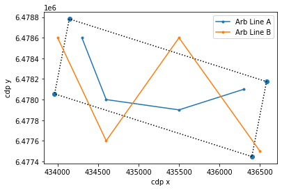
We define a line as lists of cdp_x & cdp_y points. These can be inside or outside of the survey, but obviously should intersect it in order to be useful.
[6]:
arb_line_A = (
    np.array([434300, 434600, 435500, 436300]),
    np.array([6.4786e6, 6.4780e6, 6.4779e6, 6.4781e6]),
)
arb_line_B = (
    np.array([434000, 434600, 435500, 436500]),
    np.array([6.4786e6, 6.4776e6, 6.4786e6, 6.4775e6]),
)
Let’s see how these lines are placed relative to the survey bounds. We can see A is fully enclosed whilst B has some segments outside.
[7]:
ax = volve_3d.seis.plot_bounds()
ax.plot(arb_line_A[0], arb_line_A[1], ".-", label="Arb Line A")
ax.plot(arb_line_B[0], arb_line_B[1], ".-", label="Arb Line B")
ax.legend()
[7]:
<matplotlib.legend.Legend at 0x7f6d4bb2abb0>
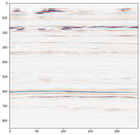
Let’s extract line A.
We specify a bin_spacing_hint which is our desired bin spacing along the line. The function use this hint to calculate the closest binspacing that maintains uniform sampling.
We have also specified the method='linear', this is the default but you can specify and method that DataArray.interp accepts
[8]:
from time import time

tic = time()
line_A = volve_3d.seis.interp_line(arb_line_A[0], arb_line_A[1], bin_spacing_hint=10)
toc = time()
print(f"That took {toc-tic} seconds")
That took 0.10650753974914551 seconds
[9]:
plt.figure(figsize=(8, 8))
plt.imshow(line_A.to_array().squeeze().T, aspect="auto", cmap="RdBu", vmin=-10, vmax=10)
[9]:
<matplotlib.image.AxesImage at 0x7f6d4be52c40>
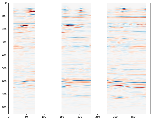
Now, let’s extract line B. Note that blank traces are inserted where the line extends outside the survey bounds.
[10]:
tic = time()
line_B = volve_3d.seis.interp_line(arb_line_B[0], arb_line_B[1], bin_spacing_hint=10)
toc = time()
print(f"That took {toc-tic} seconds")
That took 0.10834288597106934 seconds
[11]:
plt.figure(figsize=(10, 8))
plt.imshow(line_B.to_array().squeeze().T, aspect="auto", cmap="RdBu", vmin=-10, vmax=10)
[11]:
<matplotlib.image.AxesImage at 0x7f6d4bdcebb0>
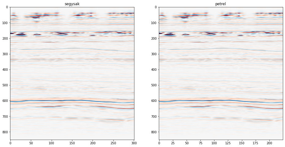
Petrel Shapefile
We have an arbitrary line geometry defined over this small survey region stored in a shape file exported from Petrel.
Let’s load that and extract an arbitrary line using segysak. We also have the seismic data extracted along that line by Petrel, so we can see how that compares.
[12]:
import shapefile
from pprint import pprint
Load the shapefile and get the list of points
[13]:
sf = shapefile.Reader(path.join("data", "arbitrary_line.shp"))
line_petrel = sf.shapes()
print(f"shapes are type {sf.shapeType} == POLYLINEZ")
print(f"There are {len(sf.shapes())} shapes in here")
print(f"The line has {len(sf.shape(0).points)} points")

points_from_shapefile = [list(t) for t in list(zip(*sf.shape(0).points))]
pprint(points_from_shapefile)
shapes are type 13 == POLYLINEZ
There are 1 shapes in here
The line has 10 points
[[434244.1111175297,
  434285.5847503422,
  434588.36941831093,
  434885.0338465618,
  435036.1407475077,
  435239.3142425297,
  435544.93789816764,
  435714.1388649335,
  435772.37332456093,
  436308.21023862343],
 [6478575.031033052,
  6478218.093533052,
  6477971.34255649,
  6477874.469884046,
  6477991.699391355,
  6478202.953884615,
  6478214.490538706,
  6478065.665258892,
  6477687.288845552,
  6477563.074001802]]
Load the segy containing the line that Petrel extracted along this geometry
[14]:
line_extracted_by_petrel_path = path.join("data", "volve10r12-full-twt-arb.sgy")
print(
    f"{line_extracted_by_petrel_path} exists: {path.exists(line_extracted_by_petrel_path)}"
)
line_extracted_by_petrel = segy_loader(
    line_extracted_by_petrel_path, **well_known_byte_locs("petrel_3d")
)
data/volve10r12-full-twt-arb.sgy exists: True
100%|██████████| 225/225 [00:00<00:00, 10.9k traces/s]
Loading as 3D
Fast direction is TRACE_SEQUENCE_FILE
Converting SEGY: 100%|██████████| 225/225 [00:00<00:00, 2.12k traces/s]
Extract the line using segysak
[15]:
tic = time()
line_extracted_by_segysak = volve_3d.seis.interp_line(
    *points_from_shapefile,
    bin_spacing_hint=10,
    line_method="linear",
    xysel_method="linear",
)
toc = time()
print(f"That took {toc-tic} seconds")
That took 0.107421875 seconds
Plot the extracted lines side by side
[16]:
fig, axs = plt.subplots(1, 2, figsize=(16, 8))

axs[0].imshow(
    line_extracted_by_segysak.to_array().squeeze().T,
    aspect="auto",
    cmap="RdBu",
    vmin=-10,
    vmax=10,
)
axs[0].set_title("segysak")
axs[1].imshow(
    line_extracted_by_petrel.to_array().squeeze().T,
    aspect="auto",
    cmap="RdBu",
    vmin=-10,
    vmax=10,
)
axs[1].set_title("petrel")
[16]:
Text(0.5, 1.0, 'petrel')
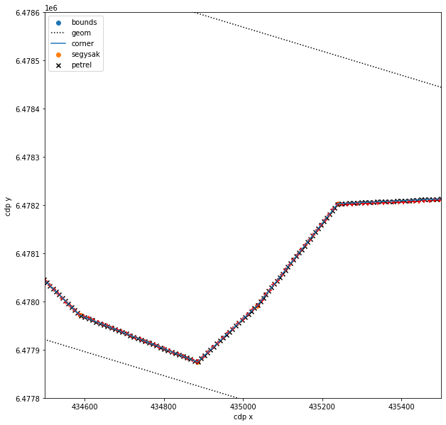
Plot the geometry, trace header locations along with the volve 3d bound box, to make sure things line up.
[17]:
plt.figure(figsize=(10, 10))
ax = volve_3d.seis.plot_bounds(ax=plt.gca())

# plot path
ax.plot(*points_from_shapefile)
ax.scatter(*points_from_shapefile)

# plot trace positons from extracted lines based on header
ax.scatter(
    line_extracted_by_segysak.cdp_x,
    line_extracted_by_segysak.cdp_y,
    marker="x",
    color="k",
)
ax.scatter(
    line_extracted_by_petrel.cdp_x,
    line_extracted_by_petrel.cdp_y,
    marker="+",
    color="r",
)

ax.set_xlim(434500, 435500)
ax.set_ylim(6477800, 6478600)
plt.legend(labels=["bounds", "geom", "corner", "segysak", "petrel"])
[17]:
<matplotlib.legend.Legend at 0x7f6d4bbdce50>
Well Paths
Well paths can also be treated as an arbitrary line. In this example we will use the Affine transform to convert well X and Y locations to the seismic local grid, and the Xarray interp method to extract a seismic trace along the well bore.
First we have to load the well bore deviation and use wellpathpy to convert it to XYZ coordinates with a higher sampling rate.
[18]:
f12_dev = pd.read_csv("data/well_f12_deviation.asc", comment="#", delim_whitespace=True)
f12_dev_pos = wpp.deviation(*f12_dev[["MD", "INCL", "AZIM_GN"]].values.T)

# depth values in MD that we want to sample the seismic cube at
new_depths = np.arange(0, f12_dev["MD"].max(), 1)

# use minimum curvature and resample to 1m interval
f12_dev_pos = f12_dev_pos.minimum_curvature().resample(new_depths)

# adjust position of deviation to local coordinates and TVDSS
f12_dev_pos.to_wellhead(
    6478566.23,
    435050.21,
    inplace=True,
)
f12_dev_pos.loc_to_tvdss(
    54.9,
    inplace=True,
)

fig, ax = plt.subplots(figsize=(10, 5))
volve_3d.seis.plot_bounds(ax=ax)
sc = ax.scatter(f12_dev_pos.easting, f12_dev_pos.northing, c=f12_dev_pos.depth, s=1)
plt.colorbar(sc, label="F12 Depth")
ax.set_aspect("equal")

We can easily sample the seismic cube by converting the positional log to iline and xline using the Affine transform for our data. We also need to convert the TVDSS values of the data to TWT (in this case we will just use a constant velocity).
In both instances we will create custom xarray.DataArray instances because this allows us to relate the coordinate systems of well samples (on the new dimension well) to the iline and xline dimensions of the cube.
[19]:
# need the inverse to go from xy to il/xl
affine = volve_3d.seis.get_affine_transform().inverted()
ilxl = affine.transform(np.dstack([f12_dev_pos.easting, f12_dev_pos.northing])[0])

f12_dev_ilxl = dict(
    iline=xr.DataArray(ilxl[:, 0], dims="well", coords={"well": range(ilxl.shape[0])}),
    xline=xr.DataArray(ilxl[:, 1], dims="well", coords={"well": range(ilxl.shape[0])}),
)

twt = xr.DataArray(
    -1.0 * f12_dev_pos.depth * 2000 / 2400,  # 2400 m/s to convert to TWT - and negate,
    dims="well",
    coords={"well": range(ilxl.shape[0])},
)

f12_dev_ilxl
[19]:
{'iline': <xarray.DataArray (well: 3520)>
 array([10150.75378715, 10150.75378715, 10150.75378715, ...,
        10127.97048764, 10127.96872176, 10127.96695588])
 Coordinates:
   * well     (well) int64 0 1 2 3 4 5 6 7 ... 3513 3514 3515 3516 3517 3518 3519,
 'xline': <xarray.DataArray (well: 3520)>
 array([2276.4813429 , 2276.4813429 , 2276.4813429 , ..., 2247.46606976,
        2247.40231314, 2247.33855653])
 Coordinates:
   * well     (well) int64 0 1 2 3 4 5 6 7 ... 3513 3514 3515 3516 3517 3518 3519}
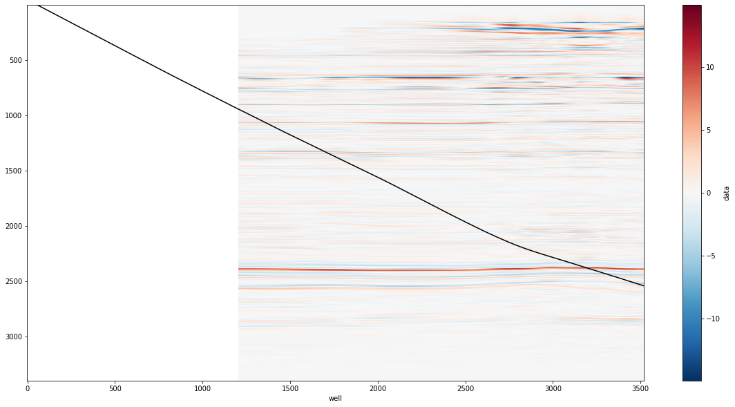
The DataArrays with the new axes can be passed to interp which will perform interpolation for us on the new dimension well.
We can also plot the well path on our seismic extracted along the well path.
[20]:
sel = volve_3d.interp(**f12_dev_ilxl)
fig, axs = plt.subplots(figsize=(20, 10))
sel.data.T.plot(ax=axs, yincrease=False)
twt.plot(color="k", ax=axs)
[20]:
[<matplotlib.lines.Line2D at 0x7f6d4895b760>]
To extract the data along the well path we just need to interpolate using the additional twt DataArray.
[21]:
well_seismic = volve_3d.interp(**f12_dev_ilxl, twt=twt)
well_seismic.data.plot()
[21]:
[<matplotlib.lines.Line2D at 0x7f6d488d0fd0>]
