Note
Get this example as a Jupyter Notebook ipynb
Merging Seismic Data Cubes
Often we receive seismic data cubes which we wish to merge that have different geometries. This workflow will guide you through the process of merging two such cubes.
[1]:
from segysak import create3d_dataset
from scipy.optimize import curve_fit
import numpy as np
import xarray as xr
import matplotlib.pyplot as plt
from matplotlib.transforms import Affine2D
from segysak import open_seisnc, create_seismic_dataset

from dask.distributed import Client

# start a dask client for processing
client = Client()
Creating some synthetic seismic surveys for us to play with. The online documentation uses a smaller example, but you can stress dask by commenting the dimension lines for smaller data and uncommenting the large desktop size volumes.
[2]:
# large desktop size merge
# i1, i2, iN = 100, 750, 651
# x1, x2, xN = 300, 1250, 951
# t1, t2, tN = 0, 1848, 463
# trans_x, trans_y = 10000, 2000

# online example size merge
i1, i2, iN = 650, 750, 101
x1, x2, xN = 1150, 1250, 101
t1, t2, tN = 0, 200, 201
trans_x, trans_y = 9350, 1680

iline = np.linspace(i1, i2, iN, dtype=int)
xline = np.linspace(x1, x2, xN, dtype=int)
twt = np.linspace(t1, t2, tN, dtype=int)

affine_survey1 = Affine2D()
affine_survey1.rotate_deg(20).translate(trans_x, trans_y)

# create an empty dataset and empty coordinates
survey_1 = create_seismic_dataset(twt=twt, iline=iline, xline=xline)
survey_1["cdp_x"] = (("iline", "xline"), np.empty((iN, xN)))
survey_1["cdp_y"] = (("iline", "xline"), np.empty((iN, xN)))

stacked_iline = survey_1.iline.broadcast_like(survey_1.cdp_x).stack(
    {"ravel": (..., "xline")}
)
stacked_xline = survey_1.xline.broadcast_like(survey_1.cdp_x).stack(
    {"ravel": (..., "xline")}
)

points = np.dstack([stacked_iline, stacked_xline])
points_xy = affine_survey1.transform(points[0])
# put xy back in stacked and unstack into survey_1
survey_1["cdp_x"] = stacked_iline.copy(data=points_xy[:, 0]).unstack()
survey_1["cdp_y"] = stacked_iline.copy(data=points_xy[:, 1]).unstack()

# and the same for survey_2 but with a different affine to survey 1
affine_survey2 = Affine2D()
affine_survey2.rotate_deg(120).translate(11000, 3000)

survey_2 = create_seismic_dataset(twt=twt, iline=iline, xline=xline)
survey_2["cdp_x"] = (("iline", "xline"), np.empty((iN, xN)))
survey_2["cdp_y"] = (("iline", "xline"), np.empty((iN, xN)))

stacked_iline = survey_1.iline.broadcast_like(survey_1.cdp_x).stack(
    {"ravel": (..., "xline")}
)
stacked_xline = survey_1.xline.broadcast_like(survey_1.cdp_x).stack(
    {"ravel": (..., "xline")}
)

points = np.dstack([stacked_iline, stacked_xline])
points_xy = affine_survey2.transform(points[0])
# put xy back in stacked and unstack into survey_1
survey_2["cdp_x"] = stacked_iline.copy(data=points_xy[:, 0]).unstack()
survey_2["cdp_y"] = stacked_iline.copy(data=points_xy[:, 1]).unstack()
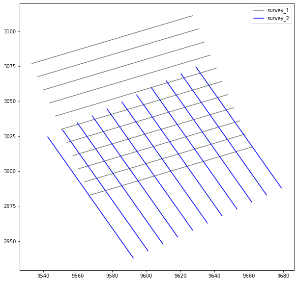
Let’s check that there is a bit of overlap between the two surveys.
[3]:
# plotting every 10th line

plt.figure(figsize=(10, 10))
survey_1_plot = plt.plot(
    survey_1.cdp_x.values[::10, ::10], survey_1.cdp_y.values[::10, ::10], color="grey"
)
survey_2_plot = plt.plot(
    survey_2.cdp_x.values[::10, ::10], survey_2.cdp_y.values[::10, ::10], color="blue"
)
# plt.aspect("equal")
plt.legend([survey_1_plot[0], survey_2_plot[0]], ["survey_1", "survey_2"])
[3]:
<matplotlib.legend.Legend at 0x7f1b00fb96a0>
Let’s output these two datasets to disk so we can use lazy loading from seisnc. If the files are large, it’s good practice to do this, because you will probably run out of memory.
We are going to fill survey one with a values of 1 and survey 2 with a value of 2, just for simplicity in this example. We also tell the dtype to be np.float32 to reduce memory usage.
[4]:
# save out with new geometry
survey_1["data"] = (
    ("iline", "xline", "twt"),
    np.full((iN, xN, tN), 1, dtype=np.float32),
)
survey_1.seisio.to_netcdf("data/survey_1.seisnc")
del survey_1
survey_2["data"] = (
    ("iline", "xline", "twt"),
    np.full((iN, xN, tN), 2, dtype=np.float32),
)
survey_2.seisio.to_netcdf("data/survey_2.seisnc")
del survey_2
How to merge two different geometries
Let us reimport the surveys we created but in a chunked (lazy) way.
[5]:
survey_1 = open_seisnc("data/survey_1.seisnc", chunks=dict(iline=10, xline=10, twt=100))
survey_2 = open_seisnc("data/survey_2.seisnc", chunks=dict(iline=10, xline=10, twt=100))
Check that the survey is chunked by looking at the printout for our datasets. Lazy and chunked data will have a dask.array<chunksize= where the values are usually displayed.
[6]:
survey_1
[6]:
<xarray.Dataset>
Dimensions:  (iline: 101, xline: 101, twt: 201)
Coordinates:
    cdp_x    (iline, xline) float64 dask.array<chunksize=(10, 10), meta=np.ndarray>
    cdp_y    (iline, xline) float64 dask.array<chunksize=(10, 10), meta=np.ndarray>
  * iline    (iline) int64 650 651 652 653 654 655 ... 745 746 747 748 749 750
  * twt      (twt) int64 0 1 2 3 4 5 6 7 8 ... 193 194 195 196 197 198 199 200
  * xline    (xline) int64 1150 1151 1152 1153 1154 ... 1246 1247 1248 1249 1250
Data variables:
    data     (iline, xline, twt) float32 dask.array<chunksize=(10, 10, 100), meta=np.ndarray>
Attributes: (12/13)
    text:
    ns:                  None
    sample_rate:         None
    measurement_system:  None
    d3_domain:           None
    epsg:                None
    ...                  ...
    corner_points_xy:    None
    source_file:         None
    srd:                 None
    datatype:            None
    percentiles:         None
coord_scalar: NoneIt will help with our other functions if we load the cdp_x and cdp_y locations into memory. This can be done using the load() method.
[7]:
survey_1["cdp_x"] = survey_1["cdp_x"].load()
survey_1["cdp_y"] = survey_1["cdp_y"].load()
survey_2["cdp_x"] = survey_2["cdp_x"].load()
survey_2["cdp_y"] = survey_2["cdp_y"].load()
[8]:
survey_1
[8]:
<xarray.Dataset>
Dimensions:  (iline: 101, xline: 101, twt: 201)
Coordinates:
    cdp_x    (iline, xline) float64 9.567e+03 9.567e+03 ... 9.628e+03 9.627e+03
    cdp_y    (iline, xline) float64 2.983e+03 2.984e+03 ... 3.11e+03 3.111e+03
  * iline    (iline) int64 650 651 652 653 654 655 ... 745 746 747 748 749 750
  * twt      (twt) int64 0 1 2 3 4 5 6 7 8 ... 193 194 195 196 197 198 199 200
  * xline    (xline) int64 1150 1151 1152 1153 1154 ... 1246 1247 1248 1249 1250
Data variables:
    data     (iline, xline, twt) float32 dask.array<chunksize=(10, 10, 100), meta=np.ndarray>
Attributes: (12/13)
    text:
    ns:                  None
    sample_rate:         None
    measurement_system:  None
    d3_domain:           None
    epsg:                None
    ...                  ...
    corner_points_xy:    None
    source_file:         None
    srd:                 None
    datatype:            None
    percentiles:         None
coord_scalar: NoneWe will also need an affine transform which converts from il/xl on survey 2 to il/xl on survey 1. This will relate the two grids to each other. Fortunately affine transforms can be added together which makes this pretty straight forward.
[9]:
ilxl2_to_ilxl1 = (
    survey_2.seis.get_affine_transform()
    + survey_1.seis.get_affine_transform().inverted()
)
Let’s check the transform to see if it makes sense. The colouring of our values by inline should be the same after the transform is applied. Cool.
[10]:
# plotting every 50th line

n = 5

fig, axs = plt.subplots(ncols=2, figsize=(20, 10))
survey_1_plot = axs[0].scatter(
    survey_1.cdp_x.values[::n, ::n],
    survey_1.cdp_y.values[::n, ::n],
    c=survey_1.iline.broadcast_like(survey_1.cdp_x).values[::n, ::n],
    s=20,
)
survey_2_plot = axs[0].scatter(
    survey_2.cdp_x.values[::n, ::n],
    survey_2.cdp_y.values[::n, ::n],
    c=survey_2.iline.broadcast_like(survey_2.cdp_x).values[::n, ::n],
    s=20,
)
plt.colorbar(survey_1_plot, ax=axs[0])
axs[0].set_aspect("equal")

axs[0].set_title("inline numbering before transform")

new_ilxl = ilxl2_to_ilxl1.transform(
    np.dstack(
        [
            survey_2.iline.broadcast_like(survey_2.cdp_x).values.ravel(),
            survey_2.xline.broadcast_like(survey_2.cdp_x).values.ravel(),
        ]
    )[0]
).reshape((survey_2.iline.size, survey_2.xline.size, 2))

survey_2.seis.calc_corner_points()
s2_corner_points_in_s1 = ilxl2_to_ilxl1.transform(survey_2.attrs["corner_points"])

print("Min Iline:", s2_corner_points_in_s1[:, 0].min(), survey_1.iline.min().values)
min_iline_combined = min(
    s2_corner_points_in_s1[:, 0].min(), survey_1.iline.min().values
)
print("Max Iline:", s2_corner_points_in_s1[:, 0].max(), survey_1.iline.max().values)
max_iline_combined = max(
    s2_corner_points_in_s1[:, 0].max(), survey_1.iline.max().values
)

print("Min Xline:", s2_corner_points_in_s1[:, 1].min(), survey_1.xline.min().values)
min_xline_combined = min(
    s2_corner_points_in_s1[:, 1].min(), survey_1.xline.min().values
)
print("Max Xline:", s2_corner_points_in_s1[:, 1].max(), survey_1.xline.max().values)
max_xline_combined = max(
    s2_corner_points_in_s1[:, 1].max(), survey_1.xline.max().values
)
print(min_iline_combined, max_iline_combined, min_xline_combined, max_xline_combined)

survey_1_plot = axs[1].scatter(
    survey_1.cdp_x.values[::n, ::n],
    survey_1.cdp_y.values[::n, ::n],
    c=survey_1.iline.broadcast_like(survey_1.cdp_x).values[::n, ::n],
    vmin=min_iline_combined,
    vmax=max_iline_combined,
    s=20,
    cmap="hsv",
)


survey_2_plot = axs[1].scatter(
    survey_2.cdp_x.values[::n, ::n],
    survey_2.cdp_y.values[::n, ::n],
    c=new_ilxl[::n, ::n, 0],
    vmin=min_iline_combined,
    vmax=max_iline_combined,
    s=20,
    cmap="hsv",
)
plt.colorbar(survey_1_plot, ax=axs[1])

axs[1].set_title("inline numbering after transform")
axs[1].set_aspect("equal")
Min Iline: 640.7135889711899 650
Max Iline: 756.5591820391251 750
Min Xline: 1099.1258403243169 1150
Max Xline: 1214.9714333922225 1250
640.7135889711899 756.5591820391251 1099.1258403243169 1250

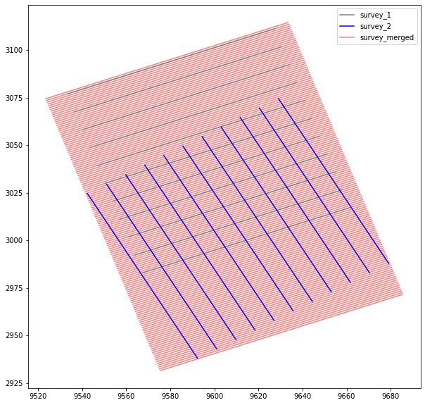
So we now have a transform that can convert ilxl from survey_2 to ilxl from survey_1 and we need to create a combined geometry for the merge. The dims need to cover the maximum range (inline, crossline) of two surveys. We are also going to use survey 1 as the base as we don’t want to have to resample two cubes, although if you have a prefered geometry you could do that (custom affine transforms per survey required).
[11]:
# create new dims
iline_step = survey_1.iline.diff("iline").mean().values
xline_step = survey_1.xline.diff("xline").mean().values

# create the new dimensions
new_iline_dim = np.arange(
    int(min_iline_combined // iline_step) * iline_step,
    int(max_iline_combined) + iline_step * 2,
    iline_step,
    dtype=np.int32,
)
new_xline_dim = np.arange(
    int(min_xline_combined // xline_step) * xline_step,
    int(max_xline_combined) + xline_step * 2,
    xline_step,
    dtype=np.int32,
)

# create a new empty dataset and a blank cdp_x for dims broadcasting
survey_comb = create_seismic_dataset(
    iline=new_iline_dim, xline=new_xline_dim, twt=survey_1.twt
)
survey_comb["cdp_x"] = (
    ("iline", "xline"),
    np.empty((new_iline_dim.size, new_xline_dim.size)),
)

# calculate the x and y using the survey 1 affine which is our base grid and reshape to the dataset grid
new_cdp_xy = affine_survey1.transform(
    np.dstack(
        [
            survey_comb.iline.broadcast_like(survey_comb.cdp_x).values.ravel(),
            survey_comb.xline.broadcast_like(survey_comb.cdp_x).values.ravel(),
        ]
    )[0]
)
new_cdp_xy_grid = new_cdp_xy.reshape((new_iline_dim.size, new_xline_dim.size, 2))

# plot to check
plt.figure(figsize=(10, 10))

survey_comb_plot = plt.plot(
    new_cdp_xy_grid[:, :, 0], new_cdp_xy_grid[:, :, 1], color="red", alpha=0.5
)
survey_1_plot = plt.plot(
    survey_1.cdp_x.values[::10, ::10], survey_1.cdp_y.values[::10, ::10], color="grey"
)
survey_2_plot = plt.plot(
    survey_2.cdp_x.values[::10, ::10], survey_2.cdp_y.values[::10, ::10], color="blue"
)

plt.legend(
    [survey_1_plot[0], survey_2_plot[0], survey_comb_plot[0]],
    ["survey_1", "survey_2", "survey_merged"],
)

# put the new x and y in the empty dataset
survey_comb["cdp_x"] = (("iline", "xline"), new_cdp_xy_grid[..., 0])
survey_comb["cdp_y"] = (("iline", "xline"), new_cdp_xy_grid[..., 1])
survey_comb = survey_comb.set_coords(("cdp_x", "cdp_y"))
Resampling survey_2 to survey_1 geometry
Resampling one dataset to another requires us to tell Xarray/dask where we want the new traces to be. First we can convert the x and y coordinates of the combined survey to the il xl of survey 2 using the affine transform of survey 2. This transform works il/xl to x and y and therefore we need it inverted.
[12]:
survey_2_new_ilxl_loc = affine_survey2.inverted().transform(new_cdp_xy)
We then need to create a sampling DataArray. If we passed the iline and cross line locations from the previous cell unfortunately Xarray would broadcast the inline and xline values against each other. The simplest way is to create a new stacked flat dimension which we can unstack into a cube later.
We also need to give it unique names so xarray doesn’t confuse the new dimensions with the old dimensions.
[13]:
flat = (
    survey_comb.rename(  # use the combined survey
        {"iline": "new_iline", "xline": "new_xline"}
    )  # renaming inline and xline so they don't confuse xarray
    .stack(
        {"flat": ("new_iline", "new_xline")}
    )  # and flatten the iline and xline axes using stack
    .flat  # return just the flat coord object which is multi-index (so we can unstack later)
)
flat
[13]:
<xarray.DataArray 'flat' (flat: 18054)>
array([(640, 1099), (640, 1100), (640, 1101), ..., (757, 1249), (757, 1250),
       (757, 1251)], dtype=object)
Coordinates:
    cdp_x      (flat) float64 9.576e+03 9.575e+03 ... 9.634e+03 9.633e+03
    cdp_y      (flat) float64 2.932e+03 2.933e+03 ... 3.114e+03 3.114e+03
  * flat       (flat) MultiIndex
  - new_iline  (flat) int64 640 640 640 640 640 640 ... 757 757 757 757 757 757
- new_xline (flat) int64 1099 1100 1101 1102 1103 ... 1248 1249 1250 1251[14]:
# create a dictionary of new coordinates to sample to. We use flat here because it will easily allow us to
# unstack the data after interpolation. It's necessary to use this flat dataset, otherwise xarray will try to
# interpolate on the cartesian product of iline and xline, which isn't really what we want.

resampling_data_arrays = dict(
    iline=xr.DataArray(survey_2_new_ilxl_loc[:, 0], dims="flat", coords={"flat": flat}),
    xline=xr.DataArray(survey_2_new_ilxl_loc[:, 1], dims="flat", coords={"flat": flat}),
)

resampling_data_arrays
[14]:
{'iline': <xarray.DataArray (flat: 18054)>
 array([653.01535386, 654.00016161, 654.98496936, ..., 780.41968002,
        781.40448778, 782.38929553])
 Coordinates:
   * flat       (flat) MultiIndex
   - new_iline  (flat) int64 640 640 640 640 640 640 ... 757 757 757 757 757 757
   - new_xline  (flat) int64 1099 1100 1101 1102 1103 ... 1248 1249 1250 1251,
 'xline': <xarray.DataArray (flat: 18054)>
 array([1267.82560706, 1267.65195888, 1267.47831071, ..., 1126.55587331,
        1126.38222513, 1126.20857695])
 Coordinates:
   * flat       (flat) MultiIndex
   - new_iline  (flat) int64 640 640 640 640 640 640 ... 757 757 757 757 757 757
   - new_xline  (flat) int64 1099 1100 1101 1102 1103 ... 1248 1249 1250 1251}
The resampling can take a while with larger cubes, so it is good to use dask and to output the cube to disk at this step. When using dask for processing it is better to output to disk regularly, as this will improve how your code runs and the overall memory usage.
If you are executing this exmample locally, the task progress can be viewed by opening the dask `client <http://localhost:8787/status>`__.
[15]:
survey_2_resamp = survey_2.interp(**resampling_data_arrays)
survey_2_resamp_newgeom = (
    survey_2_resamp.drop_vars(("iline", "xline"))
    .unstack("flat")
    .rename({"new_iline": "iline", "new_xline": "xline"})
    .data
)
survey_2_resamp_newgeom.to_netcdf("data/survey_2_1.nc", compute=True, engine="h5netcdf")
Combining Cubes
The last step is combining the cube is to load the two datasets to be combined and concatenate them together along a new axis. This will simplify reduction processes later.
[16]:
survey_2_resamp_newgeom = xr.open_dataarray(
    "data/survey_2_1.nc", chunks=dict(iline=10, xline=10, twt=100), engine="h5netcdf"
)
[17]:
survey_2_resamp_newgeom.expand_dims({"survey": [2]})
[17]:
<xarray.DataArray 'data' (survey: 1, twt: 201, iline: 118, xline: 153)>
dask.array<broadcast_to, shape=(1, 201, 118, 153), dtype=float32, chunksize=(1, 100, 10, 10), chunktype=numpy.ndarray>
Coordinates:
  * survey   (survey) int64 2
    cdp_x    (iline, xline) float64 dask.array<chunksize=(10, 10), meta=np.ndarray>
    cdp_y    (iline, xline) float64 dask.array<chunksize=(10, 10), meta=np.ndarray>
  * iline    (iline) int64 640 641 642 643 644 645 ... 752 753 754 755 756 757
  * twt      (twt) int64 0 1 2 3 4 5 6 7 8 ... 193 194 195 196 197 198 199 200
* xline (xline) int64 1099 1100 1101 1102 1103 ... 1247 1248 1249 1250 1251[18]:
# concatenate survey with new dimension "survey".
survey_comb["data"] = xr.concat([survey_1.data, survey_2_resamp_newgeom], "survey")
/opt/hostedtoolcache/Python/3.8.12/x64/lib/python3.8/site-packages/dask/array/core.py:4571: PerformanceWarning: Increasing number of chunks by factor of 11
  result = blockwise(
[19]:
survey_comb
[19]:
<xarray.Dataset>
Dimensions:  (iline: 118, xline: 153, twt: 201, survey: 2)
Coordinates:
  * iline    (iline) int64 640 641 642 643 644 645 ... 752 753 754 755 756 757
  * xline    (xline) int64 1099 1100 1101 1102 1103 ... 1247 1248 1249 1250 1251
  * twt      (twt) int64 0 1 2 3 4 5 6 7 8 ... 193 194 195 196 197 198 199 200
    cdp_x    (iline, xline) float64 9.576e+03 9.575e+03 ... 9.634e+03 9.633e+03
    cdp_y    (iline, xline) float64 2.932e+03 2.933e+03 ... 3.114e+03 3.114e+03
Dimensions without coordinates: survey
Data variables:
    data     (survey, iline, xline, twt) float32 dask.array<chunksize=(1, 10, 10, 100), meta=np.ndarray>
Attributes: (12/13)
    ns:                  None
    sample_rate:         None
    text:                None
    measurement_system:  None
    d3_domain:           None
    epsg:                None
    ...                  ...
    corner_points_xy:    None
    source_file:         None
    srd:                 None
    datatype:            None
    percentiles:         None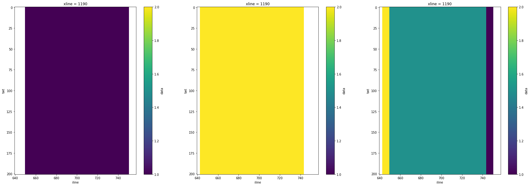
coord_scalar: NoneWe can check the merged surveys by looking at some plots. If we select just the first survey the values will be 1. If we select just the second survey the values will be 2. And if we take the mean along the survey dimension, then where the surveys overlap the values will be 1.5.
For seismic data, a better form of conditioning and reduction might be required for merging traces together to ensure a smoother seam.
[20]:
sel = survey_comb.sel(xline=1190)

fig, axs = plt.subplots(ncols=3, figsize=(30, 10))

sel.isel(survey=0).data.T.plot(ax=axs[0], yincrease=False, vmin=1, vmax=2)
sel.isel(survey=1).data.T.plot(ax=axs[1], yincrease=False, vmin=1, vmax=2)
sel.data.mean("survey").T.plot(ax=axs[2], yincrease=False, vmin=1, vmax=2)
[20]:
<matplotlib.collections.QuadMesh at 0x7f1b001cc610>
[21]:
survey_comb.twt
[21]:
<xarray.DataArray 'twt' (twt: 201)>
array([  0,   1,   2, ..., 198, 199, 200])
Coordinates:
  * twt      (twt) int64 0 1 2 3 4 5 6 7 8 ... 193 194 195 196 197 198 199 200
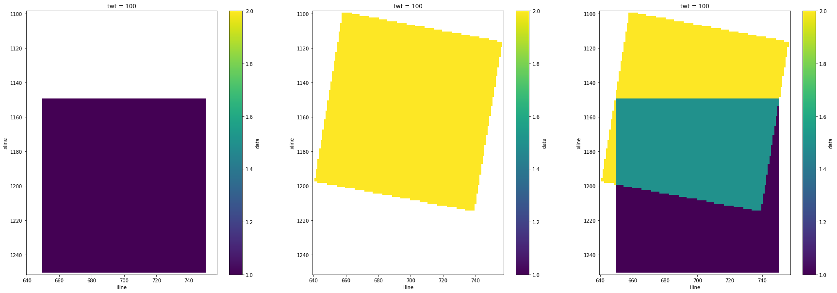
And if we inspect a time slice.
[22]:
sel = survey_comb.sel(twt=100)

fig, axs = plt.subplots(ncols=3, figsize=(30, 10))

sel.isel(survey=0).data.T.plot(ax=axs[0], yincrease=False, vmin=1, vmax=2)
sel.isel(survey=1).data.T.plot(ax=axs[1], yincrease=False, vmin=1, vmax=2)
sel.data.mean("survey").T.plot(ax=axs[2], yincrease=False, vmin=1, vmax=2)
[22]:
<matplotlib.collections.QuadMesh at 0x7f1ae05141f0>
[ ]: