Note
Get this example as a Jupyter Notebook ipynb
[ ]:
SEGY-SAK Basics
segysak offers a number of utilities to create and load seismic data using xarray and segyio. In general segysak uses xarray.Dataset to store the data and provides an interface to additional seismic specific functionality by adding the .seis and .seisio names-spaces to an xarray.Dataset (just dataset from now on). That sounds complicated but let us walk through some examples together.
Creating empty 3D geometry
In segysak we use the term seisnc to refer to a dataset which is compatible with segysak’s functionality and which has the additional names spaces registered with xarray, for all intensive purposes it is an xarray.Dataset but with defined dimensions and coordinates and some extended functionality. The seisnc dimensions are defined depending on what type of seismic it is (2D, 3D, gathers, etc.)
To create an empty 3D instance of seisnc use the create3d_dataset. The function creates a new seisnc based upon definitions for the dimensions, iline numbering, xline numbering and the vertical sampling.
[1]:
import matplotlib.pyplot as plt

%matplotlib inline

from segysak import create3d_dataset

# dims iline, xline, vert
dims = (10, 5, 1000)

new_seisnc = create3d_dataset(
    dims,
    first_iline=1,
    iline_step=2,
    first_xline=10,
    xline_step=1,
    first_sample=0,
    sample_rate=1,
    vert_domain="TWT",
)
new_seisnc
[1]:
<xarray.Dataset>
Dimensions:  (iline: 10, xline: 5, twt: 1000)
Coordinates:
  * iline    (iline) int64 1 3 5 7 9 11 13 15 17 19
  * xline    (xline) int64 10 11 12 13 14
  * twt      (twt) int64 0 1 2 3 4 5 6 7 8 ... 992 993 994 995 996 997 998 999
Data variables:
    *empty*
Attributes: (12/13)
    ns:                  None
    sample_rate:         1
    text:                SEGY-SAK Create 3D Dataset
    measurement_system:  None
    d3_domain:           TWT
    epsg:                None
    ...                  ...
    corner_points_xy:    None
    source_file:         None
    srd:                 None
    datatype:            None
    percentiles:         None
coord_scalar: NoneDimension based selection and transformation
As you can see from the print out of the previous cell, we have three dimensions in this dataset. They are iline, xline and twt (although the order, number and names might change depending on the make up of our volume). The ordering isn’t import to xarray because it uses labels, and accessing data is done using these labels rather than indexing directly into the data like numpy. xarray also makes it further convenient by allowing us to select based on the dimension values
using the .sel method with tools for selecting nearest or ranges as well. If necessary you can also select by index using the .isel method.
[2]:
# select iline value 9
xarray_selection = new_seisnc.sel(iline=9)
# select xline value 12
xarray_selection = new_seisnc.sel(xline=12)
# select iline and xline intersection point
xarray_selection = new_seisnc.sel(iline=9, xline=12)
# key error
# xarray_selection = new_seisnc.sel(twt=8.5)
# select nearest twt slice
xarray_selection = new_seisnc.sel(twt=8.5, method="nearest")
# select a range
xarray_selection = new_seisnc.sel(iline=[9, 11, 13])
# select a subcube
# also slices can be used to select ranges as if they were indices!
xarray_selection = new_seisnc.sel(iline=slice(9, 13), xline=[10, 11, 12])
# index selection principles are similar
xarray_selection = new_seisnc.sel(iline=slice(1, 4))

# putting it altogether to extract a sub-cropped horizon slice at odd interval
xarray_selection = new_seisnc.sel(
    twt=8.5, iline=new_seisnc.iline[:4], xline=[10, 12], method="nearest"
)
xarray_selection
[2]:
<xarray.Dataset>
Dimensions:  (iline: 4, xline: 2)
Coordinates:
  * iline    (iline) int64 1 3 5 7
  * xline    (xline) int64 10 12
    twt      int64 9
Data variables:
    *empty*
Attributes: (12/13)
    ns:                  None
    sample_rate:         1
    text:                SEGY-SAK Create 3D Dataset
    measurement_system:  None
    d3_domain:           TWT
    epsg:                None
    ...                  ...
    corner_points_xy:    None
    source_file:         None
    srd:                 None
    datatype:            None
    percentiles:         None
coord_scalar: NoneCoordinates Selection
Usually for seismic the X and Y coordinates labelled cdp_x and cdp_y in seisnc are rotated and scaled relative to the grid geometry and now seisnc dimensions iline, xline and twt. For xarray this means you cannot use the .sel and .isel methods to select data for cdp_x and cdp_y. segysak is developing more natural interfaces to access data using X and Y coordinates and this is available through the seisnc.seis namespace, covered in other examples.
Adding data to an empty seisnc
Because xarray needs to understand the dimensions of any data you assign it must be explicitly communicated either via labels or creating an xarray.DataArray first.
[3]:
# get the dims
dims = new_seisnc.dims
print(dims)
dkeys = ("xline", "iline", "twt")
dsize = [dims[key] for key in dkeys]
print("keys:", dkeys, "sizes:", dsize)
Frozen({'iline': 10, 'xline': 5, 'twt': 1000})
keys: ('xline', 'iline', 'twt') sizes: [5, 10, 1000]
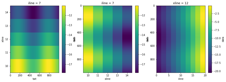
[4]:
import numpy as np

# create some data and the dimension shapes
xline_, iline_, twt_ = np.meshgrid(new_seisnc.iline, new_seisnc.xline, new_seisnc.twt)
data = np.sin(twt_ / 100) + 2 * iline_ * np.cos(xline_ / 20 + 10)

# assign the data to dataset by passing in a tuple of the dimension keys and the new data
new_seisnc["data"] = (dkeys, data)

fig, axs = plt.subplots(ncols=3, figsize=(15, 5))

# axes are wrong for seismic
new_seisnc.data.sel(iline=7).plot(ax=axs[0])

# rotate the cube
new_seisnc.data.transpose("twt", "iline", "xline").sel(iline=7).plot(
    ax=axs[1], yincrease=False
)

# xline is the same?
new_seisnc.data.transpose("twt", "iline", "xline").isel(xline=2).plot(
    ax=axs[2], yincrease=False
)
[4]:
<matplotlib.collections.QuadMesh at 0x7f97d1bd84c0>
Other Useful Methods
Accessing the coordinates or data as a numpy array.
[5]:
# Data can be dropped out of xarray but you then need to manage the coordinates and the dimension
# labels

new_seisnc.iline.values
[5]:
array([ 1, 3, 5, 7, 9, 11, 13, 15, 17, 19])
xarray.Dataset and DataArray have lots of great built in methods in addition to plot.
[6]:
print(new_seisnc.data.mean())
<xarray.DataArray 'data' ()>
array(-10.76364169)
[7]:
print(new_seisnc.data.max())
<xarray.DataArray 'data' ()>
array(0.08882943)
numpy functions also work on xarray objects but this returns a new DataArray not a ndarray.
[8]:
print(np.sum(new_seisnc.data))
<xarray.DataArray 'data' ()>
array(-538182.08430941)
With xarray you can apply operations along 1 or more dimensions to reduce the dataset. This could be useful for collapsing gathers for example by applying the mean along the offset dimension. Here we combine a numpy operation abs which returns an DataArray and then sum along the time dimension to create a grid without the time dimension. Along with using masks this is a fundamental building block for performing horizonal sculpting.
[9]:
map_data = np.abs(new_seisnc.data).sum(dim="twt")
img = map_data.plot()

Sometimes we need to modify the dimensions because they were read wrong or to scale them. Modify your dimension from the seisnc and then put it back using assign_coords.
[10]:
new_seisnc.assign_coords(iline=new_seisnc.iline * 10, twt=new_seisnc.twt + 1500)
[10]:
<xarray.Dataset>
Dimensions:  (iline: 10, xline: 5, twt: 1000)
Coordinates:
  * iline    (iline) int64 10 30 50 70 90 110 130 150 170 190
  * xline    (xline) int64 10 11 12 13 14
  * twt      (twt) int64 1500 1501 1502 1503 1504 ... 2495 2496 2497 2498 2499
Data variables:
    data     (xline, iline, twt) float64 -16.22 -16.21 -16.2 ... -1.803 -1.811
Attributes: (12/13)
    ns:                  None
    sample_rate:         1
    text:                SEGY-SAK Create 3D Dataset
    measurement_system:  None
    d3_domain:           TWT
    epsg:                None
    ...                  ...
    corner_points_xy:    None
    source_file:         None
    srd:                 None
    datatype:            None
    percentiles:         None
    coord_scalar:        None