Note
Get this example as a Jupyter Notebook ipynb
Quick Overview
Here you can find some quick examples of what you can do with segysak. For more details refer to the examples.
The library is imported as segysak and the loaded xarray objects are compatible with numpy and matplotlib.
The cropped volume from the Volve field in the North Sea (made available by Equinor) is used for this example, and all the examples and data in this documentation are available from the examples folder of the Github respository.
[2]:
import matplotlib.pyplot as plt
import pathlib
[3]:
V3D_path = pathlib.Path("data/volve10r12-full-twt-sub3d.sgy")
print("3D", V3D_path, V3D_path.exists())
3D data/volve10r12-full-twt-sub3d.sgy True
Scan SEGY headers
A basic operation would be to check the text header included in the SEG-Y file. The get_segy_texthead function accounts for commong encoding issues and returns the header as a text string.
[4]:
from segysak.segy import get_segy_texthead

get_segy_texthead(V3D_path)
[4]:
Text Header
C 1 SEGY OUTPUT FROM Petrel 2017.2 Saturday, June 06 2020 10:15:00
C 2 Name: ST10010ZDC12-PZ-PSDM-KIRCH-FULL-T.MIG_FIN.POST_STACK.3D.JS-017534
ÝCroC 3
C 4 First inline: 10090 Last inline: 10150
C 5 First xline: 2150 Last xline: 2351
C 6 CRS: ED50-UTM31 ("MENTOR:ED50-UTM31:European 1950 Based UTM, Zone 31 North,
C 7 X min: 433955.09 max: 436589.56 delta: 2634.47
C 8 Y min: 6477439.46 max: 6478790.23 delta: 1350.77
C 9 Time min: -3402.00 max: -2.00 delta: 3400.00
C10 Lat min: 58.25'52.8804"N max: 58.26'37.9493"N delta: 0.00'45.0689"
C11 Long min: 1.52'7.1906"E max: 1.54'50.9616"E delta: 0.02'43.7710"
C12 Trace min: -3400.00 max: -4.00 delta: 3396.00
C13 Seismic (template) min: -58.55 max: 54.55 delta: 113.10
C14 Amplitude (data) min: -58.55 max: 54.55 delta: 113.10
C15 Trace sample format: IEEE floating point
C16 Coordinate scale factor: 100.00000
C17
C18 Binary header locations:
C19 Sample interval : bytes 17-18
C20 Number of samples per trace : bytes 21-22
C21 Trace date format : bytes 25-26
C22
C23 Trace header locations:
C24 Inline number : bytes 5-8
C25 Xline number : bytes 21-24
C26 Coordinate scale factor : bytes 71-72
C27 X coordinate : bytes 73-76
C28 Y coordinate : bytes 77-80
C29 Trace start time/depth : bytes 109-110
C30 Number of samples per trace : bytes 115-116
C31 Sample interval : bytes 117-118
C32
C33
C34
C35
C36
C37
C38
C39
C40 END EBCDIC
If you need to investigate the trace header data more deeply, then segy_header_scan can be used to report basic statistic of each byte position for a limited number of traces.
segy_header_scan returns a pandas.DataFrame. To see the full DataFrame use the pandas option_context manager.
[5]:
from segysak.segy import segy_header_scan

scan = segy_header_scan(V3D_path)
scan
[5]:
| byte_loc | count | mean | std | min | 25% | 50% | 75% | max | |
|---|---|---|---|---|---|---|---|---|---|
| TRACE_SEQUENCE_LINE | 1 | 1000.0 | 100.54 | 57.831072 | 1.0 | 50.75 | 100.5 | 150.25 | 202.0 |
| TRACE_SEQUENCE_FILE | 5 | 1000.0 | 10091.98 | 1.407687 | 10090.0 | 10091.00 | 10092.0 | 10093.00 | 10094.0 |
| FieldRecord | 9 | 1000.0 | 10091.98 | 1.407687 | 10090.0 | 10091.00 | 10092.0 | 10093.00 | 10094.0 |
| TraceNumber | 13 | 1000.0 | 100.54 | 57.831072 | 1.0 | 50.75 | 100.5 | 150.25 | 202.0 |
| EnergySourcePoint | 17 | 1000.0 | 0.00 | 0.000000 | 0.0 | 0.00 | 0.0 | 0.00 | 0.0 |
| ... | ... | ... | ... | ... | ... | ... | ... | ... | ... |
| SourceEnergyDirectionMantissa | 219 | 1000.0 | 0.00 | 0.000000 | 0.0 | 0.00 | 0.0 | 0.00 | 0.0 |
| SourceEnergyDirectionExponent | 223 | 1000.0 | 0.00 | 0.000000 | 0.0 | 0.00 | 0.0 | 0.00 | 0.0 |
| SourceMeasurementMantissa | 225 | 1000.0 | 0.00 | 0.000000 | 0.0 | 0.00 | 0.0 | 0.00 | 0.0 |
| SourceMeasurementExponent | 229 | 1000.0 | 0.00 | 0.000000 | 0.0 | 0.00 | 0.0 | 0.00 | 0.0 |
| SourceMeasurementUnit | 231 | 1000.0 | 0.00 | 0.000000 | 0.0 | 0.00 | 0.0 | 0.00 | 0.0 |
89 rows × 9 columns
The header report can also be reduced by filtering blank byte locations. Here we use the standard deviation std to filter away blank values which can help us to understand the composition of the data.
For instance, key values like trace UTM coordinates are located in bytes 73 for X & 77 for Y. We can also see the byte positions of the local grid for INLINE_3D in byte 189 and for CROSSLINE_3D in byte 193.
[6]:
scan[scan["std"] > 0]
[6]:
| byte_loc | count | mean | std | min | 25% | 50% | 75% | max | |
|---|---|---|---|---|---|---|---|---|---|
| TRACE_SEQUENCE_LINE | 1 | 1000.0 | 1.005400e+02 | 57.831072 | 1.0 | 5.075000e+01 | 100.5 | 1.502500e+02 | 202.0 |
| TRACE_SEQUENCE_FILE | 5 | 1000.0 | 1.009198e+04 | 1.407687 | 10090.0 | 1.009100e+04 | 10092.0 | 1.009300e+04 | 10094.0 |
| FieldRecord | 9 | 1000.0 | 1.009198e+04 | 1.407687 | 10090.0 | 1.009100e+04 | 10092.0 | 1.009300e+04 | 10094.0 |
| TraceNumber | 13 | 1000.0 | 1.005400e+02 | 57.831072 | 1.0 | 5.075000e+01 | 100.5 | 1.502500e+02 | 202.0 |
| CDP | 21 | 1000.0 | 2.249540e+03 | 57.831072 | 2150.0 | 2.199750e+03 | 2249.5 | 2.299250e+03 | 2351.0 |
| SourceX | 73 | 1000.0 | 4.351992e+07 | 70152.496037 | 43396267.0 | 4.345933e+07 | 43519976.5 | 4.358062e+07 | 43641261.0 |
| SourceY | 77 | 1000.0 | 6.477772e+08 | 17532.885301 | 647744704.0 | 6.477622e+08 | 647777222.0 | 6.477923e+08 | 647809133.0 |
| CDP_X | 181 | 1000.0 | 4.351992e+07 | 70152.496037 | 43396267.0 | 4.345933e+07 | 43519976.5 | 4.358062e+07 | 43641261.0 |
| CDP_Y | 185 | 1000.0 | 6.477772e+08 | 17532.885301 | 647744704.0 | 6.477622e+08 | 647777222.0 | 6.477923e+08 | 647809133.0 |
| INLINE_3D | 189 | 1000.0 | 1.009198e+04 | 1.407687 | 10090.0 | 1.009100e+04 | 10092.0 | 1.009300e+04 | 10094.0 |
| CROSSLINE_3D | 193 | 1000.0 | 2.249540e+03 | 57.831072 | 2150.0 | 2.199750e+03 | 2249.5 | 2.299250e+03 | 2351.0 |
To retreive the raw header content use segy_header_scrape. Setting partial_scan=None will return the full dataframe of trace header information.
[7]:
from segysak.segy import segy_header_scrape

scrape = segy_header_scrape(V3D_path, partial_scan=1000)
scrape
[7]:
| TRACE_SEQUENCE_LINE | TRACE_SEQUENCE_FILE | FieldRecord | TraceNumber | EnergySourcePoint | CDP | CDP_TRACE | TraceIdentificationCode | NSummedTraces | NStackedTraces | ... | TransductionConstantPower | TransductionUnit | TraceIdentifier | ScalarTraceHeader | SourceType | SourceEnergyDirectionMantissa | SourceEnergyDirectionExponent | SourceMeasurementMantissa | SourceMeasurementExponent | SourceMeasurementUnit | |
|---|---|---|---|---|---|---|---|---|---|---|---|---|---|---|---|---|---|---|---|---|---|
| 0 | 1 | 10090 | 10090 | 1 | 0 | 2150 | 1 | 1 | 0 | 0 | ... | 0 | 0 | 0 | 0 | 0 | 0 | 0 | 0 | 0 | 0 |
| 1 | 2 | 10090 | 10090 | 2 | 0 | 2151 | 1 | 1 | 0 | 0 | ... | 0 | 0 | 0 | 0 | 0 | 0 | 0 | 0 | 0 | 0 |
| 2 | 3 | 10090 | 10090 | 3 | 0 | 2152 | 1 | 1 | 0 | 0 | ... | 0 | 0 | 0 | 0 | 0 | 0 | 0 | 0 | 0 | 0 |
| 3 | 4 | 10090 | 10090 | 4 | 0 | 2153 | 1 | 1 | 0 | 0 | ... | 0 | 0 | 0 | 0 | 0 | 0 | 0 | 0 | 0 | 0 |
| 4 | 5 | 10090 | 10090 | 5 | 0 | 2154 | 1 | 1 | 0 | 0 | ... | 0 | 0 | 0 | 0 | 0 | 0 | 0 | 0 | 0 | 0 |
| ... | ... | ... | ... | ... | ... | ... | ... | ... | ... | ... | ... | ... | ... | ... | ... | ... | ... | ... | ... | ... | ... |
| 995 | 188 | 10094 | 10094 | 188 | 0 | 2337 | 1 | 1 | 0 | 0 | ... | 0 | 0 | 0 | 0 | 0 | 0 | 0 | 0 | 0 | 0 |
| 996 | 189 | 10094 | 10094 | 189 | 0 | 2338 | 1 | 1 | 0 | 0 | ... | 0 | 0 | 0 | 0 | 0 | 0 | 0 | 0 | 0 | 0 |
| 997 | 190 | 10094 | 10094 | 190 | 0 | 2339 | 1 | 1 | 0 | 0 | ... | 0 | 0 | 0 | 0 | 0 | 0 | 0 | 0 | 0 | 0 |
| 998 | 191 | 10094 | 10094 | 191 | 0 | 2340 | 1 | 1 | 0 | 0 | ... | 0 | 0 | 0 | 0 | 0 | 0 | 0 | 0 | 0 | 0 |
| 999 | 192 | 10094 | 10094 | 192 | 0 | 2341 | 1 | 1 | 0 | 0 | ... | 0 | 0 | 0 | 0 | 0 | 0 | 0 | 0 | 0 | 0 |
1000 rows × 89 columns
Load SEG-Y data
All SEGY (2D, 2D gathers, 3D & 3D gathers) are ingested into xarray.Dataset objects through the segy_loader function. It is best to be explicit about the byte locations of key information but segy_loader can attempt to guess the shape of your dataset. Some standard byte positions are defined in the well_known_bytes function and others can be added via pull requests to the Github repository if desired.
[8]:
from segysak.segy import segy_loader, well_known_byte_locs

V3D = segy_loader(V3D_path, iline=189, xline=193, cdpx=73, cdpy=77, vert_domain="TWT")
V3D
Loading as 3D
Fast direction is CROSSLINE_3D
[8]:
<xarray.Dataset>
Dimensions:  (iline: 61, twt: 850, xline: 202)
Coordinates:
  * iline    (iline) int64 10090 10091 10092 10093 ... 10147 10148 10149 10150
  * xline    (xline) int64 2150 2151 2152 2153 2154 ... 2347 2348 2349 2350 2351
  * twt      (twt) float64 4.0 8.0 12.0 16.0 ... 3.392e+03 3.396e+03 3.4e+03
    cdp_x    (iline, xline) float32 4.364e+05 4.364e+05 ... 4.342e+05 4.341e+05
    cdp_y    (iline, xline) float32 6.477e+06 6.477e+06 ... 6.479e+06 6.479e+06
Data variables:
    data     (iline, xline, twt) float32 0.02057 0.02204 0.01966 ... 0.0 0.0 0.0
Attributes:
    ns:                  None
    sample_rate:         4.0
    text:                C 1 SEGY OUTPUT FROM Petrel 2017.2 Saturday, June 06...
    measurement_system:  m
    d3_domain:           None
    epsg:                None
    corner_points:       None
    corner_points_xy:    None
    source_file:         volve10r12-full-twt-sub3d.sgy
    srd:                 None
    datatype:            None
    percentiles:         [-6.971982623347994, -6.520540334073793, -1.49142619...
coord_scalar: -100.0- iline: 61
- twt: 850
- xline: 202
- iline(iline)int6410090 10091 10092 ... 10149 10150
array([10090, 10091, 10092, 10093, 10094, 10095, 10096, 10097, 10098, 10099, 10100, 10101, 10102, 10103, 10104, 10105, 10106, 10107, 10108, 10109, 10110, 10111, 10112, 10113, 10114, 10115, 10116, 10117, 10118, 10119, 10120, 10121, 10122, 10123, 10124, 10125, 10126, 10127, 10128, 10129, 10130, 10131, 10132, 10133, 10134, 10135, 10136, 10137, 10138, 10139, 10140, 10141, 10142, 10143, 10144, 10145, 10146, 10147, 10148, 10149, 10150]) - xline(xline)int642150 2151 2152 ... 2349 2350 2351
array([2150, 2151, 2152, ..., 2349, 2350, 2351])
- twt(twt)float644.0 8.0 12.0 ... 3.396e+03 3.4e+03
array([ 4., 8., 12., ..., 3392., 3396., 3400.])
- cdp_x(iline, xline)float324.364e+05 4.364e+05 ... 4.341e+05
array([[436400.5 , 436388.38, 436376.22, ..., 433986.9 , 433974.78, 433962.66], [436403.5 , 436391.38, 436379.28, ..., 433989.94, 433977.84, 433965.66], [436406.56, 436394.44, 436382.3 , ..., 433992.94, 433980.84, 433968.72], ..., [436575.9 , 436563.78, 436551.66, ..., 434162.3 , 434150.2 , 434138.06], [436578.94, 436566.84, 436554.72, ..., 434165.34, 434153.22, 434141.12], [436582. , 436569.84, 436557.72, ..., 434168.38, 434156.22, 434144.12]], dtype=float32) - cdp_y(iline, xline)float326.477e+06 6.477e+06 ... 6.479e+06
array([[6477447. , 6477450. , 6477452.5, ..., 6478048.5, 6478051.5,
        6478055. ],
       [6477459. , 6477462.5, 6477465. , ..., 6478060.5, 6478064. ,
        6478067. ],
       [6477471. , 6477474.5, 6477477. , ..., 6478073. , 6478076. ,
        6478079. ],
       ...,
       [6478150.5, 6478153.5, 6478156.5, ..., 6478752.5, 6478755. ,
        6478758.5],
       [6478162.5, 6478165.5, 6478169. , ..., 6478764.5, 6478767. ,
        6478770.5],
       [6478174.5, 6478178. , 6478181. , ..., 6478776. , 6478779.5,
        6478782.5]], dtype=float32)
- data(iline, xline, twt)float320.02057 0.02204 0.01966 ... 0.0 0.0
array([[[ 2.05745399e-02,  2.20407024e-02,  1.96589418e-02, ...,
          0.00000000e+00,  0.00000000e+00,  0.00000000e+00],
        [ 1.23256370e-02,  1.59417503e-02,  1.38800517e-02, ...,
          0.00000000e+00,  0.00000000e+00,  0.00000000e+00],
        [-1.63372169e-05,  4.92771342e-03,  3.24293785e-03, ...,
          0.00000000e+00,  0.00000000e+00,  0.00000000e+00],
        ...,
        [ 5.47898412e-02,  5.22681139e-02,  5.00054434e-02, ...,
          0.00000000e+00,  0.00000000e+00,  0.00000000e+00],
        [ 6.27492070e-02,  6.00568764e-02,  5.75365834e-02, ...,
          0.00000000e+00,  0.00000000e+00,  0.00000000e+00],
        [ 6.91987872e-02,  6.67222738e-02,  6.40410781e-02, ...,
          0.00000000e+00,  0.00000000e+00,  0.00000000e+00]],

       [[-3.46487835e-02, -3.38801444e-02, -3.20093483e-02, ...,
          0.00000000e+00,  0.00000000e+00,  0.00000000e+00],
        [-4.10056897e-02, -4.02579159e-02, -3.83855253e-02, ...,
          0.00000000e+00,  0.00000000e+00,  0.00000000e+00],
        [-5.01492284e-02, -4.94211540e-02, -4.75146063e-02, ...,
          0.00000000e+00,  0.00000000e+00,  0.00000000e+00],
...
          0.00000000e+00,  0.00000000e+00,  0.00000000e+00],
        [-8.89039040e-03, -9.03325155e-03, -8.77474993e-03, ...,
          0.00000000e+00,  0.00000000e+00,  0.00000000e+00],
        [-8.80905986e-03, -9.18869302e-03, -8.81006569e-03, ...,
          0.00000000e+00,  0.00000000e+00,  0.00000000e+00]],

       [[ 2.17335932e-02,  1.93170868e-02,  2.07530260e-02, ...,
          0.00000000e+00,  0.00000000e+00,  0.00000000e+00],
        [ 2.12477669e-02,  1.89855732e-02,  2.04903930e-02, ...,
          0.00000000e+00,  0.00000000e+00,  0.00000000e+00],
        [ 2.13435888e-02,  1.91475898e-02,  2.07546689e-02, ...,
          0.00000000e+00,  0.00000000e+00,  0.00000000e+00],
        ...,
        [ 6.19068742e-03,  5.15908375e-03,  6.23933598e-03, ...,
          0.00000000e+00,  0.00000000e+00,  0.00000000e+00],
        [ 7.53349811e-03,  6.49160147e-03,  7.51641765e-03, ...,
          0.00000000e+00,  0.00000000e+00,  0.00000000e+00],
        [ 9.05360654e-03,  7.92511553e-03,  8.82008299e-03, ...,
          0.00000000e+00,  0.00000000e+00,  0.00000000e+00]]],
      dtype=float32)
- ns :
- None
- sample_rate :
- 4.0
- text :
- C 1 SEGY OUTPUT FROM Petrel 2017.2 Saturday, June 06 2020 10:15:00 C 2 Name: ST10010ZDC12-PZ-PSDM-KIRCH-FULL-T.MIG_FIN.POST_STACK.3D.JS-017534 ÝCroC 3 C 4 First inline: 10090 Last inline: 10150 C 5 First xline: 2150 Last xline: 2351 C 6 CRS: ED50-UTM31 ("MENTOR:ED50-UTM31:European 1950 Based UTM, Zone 31 North, C 7 X min: 433955.09 max: 436589.56 delta: 2634.47 C 8 Y min: 6477439.46 max: 6478790.23 delta: 1350.77 C 9 Time min: -3402.00 max: -2.00 delta: 3400.00 C10 Lat min: 58.25'52.8804"N max: 58.26'37.9493"N delta: 0.00'45.0689" C11 Long min: 1.52'7.1906"E max: 1.54'50.9616"E delta: 0.02'43.7710" C12 Trace min: -3400.00 max: -4.00 delta: 3396.00 C13 Seismic (template) min: -58.55 max: 54.55 delta: 113.10 C14 Amplitude (data) min: -58.55 max: 54.55 delta: 113.10 C15 Trace sample format: IEEE floating point C16 Coordinate scale factor: 100.00000 C17 C18 Binary header locations: C19 Sample interval : bytes 17-18 C20 Number of samples per trace : bytes 21-22 C21 Trace date format : bytes 25-26 C22 C23 Trace header locations: C24 Inline number : bytes 5-8 C25 Xline number : bytes 21-24 C26 Coordinate scale factor : bytes 71-72 C27 X coordinate : bytes 73-76 C28 Y coordinate : bytes 77-80 C29 Trace start time/depth : bytes 109-110 C30 Number of samples per trace : bytes 115-116 C31 Sample interval : bytes 117-118 C32 C33 C34 C35 C36 C37 C38 C39 C40 END EBCDIC
- measurement_system :
- m
- d3_domain :
- None
- epsg :
- None
- corner_points :
- None
- corner_points_xy :
- None
- source_file :
- volve10r12-full-twt-sub3d.sgy
- srd :
- None
- datatype :
- None
- percentiles :
- [-6.971982623347994, -6.520540334073793, -1.4914261935601356, -5.19284718476843e-05, 1.4461416544023797, 6.346408873777661, 6.888088920417217]
- coord_scalar :
- -100.0
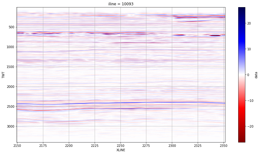
Visualising data
xarray objects use smart label based indexing techniques to retreive subsets of data. More details on xarray techniques for segysak are covered in the examples, but this demonstrates a general syntax for selecting data by label with xarray. Plottnig is done by matploblib and xarray selections can be passed to normal matplotlib.pyplot functions.
[9]:
fig, ax1 = plt.subplots(ncols=1, figsize=(15, 8))
iline_sel = 10093
V3D.data.transpose("twt", "iline", "xline", transpose_coords=True).sel(
    iline=iline_sel
).plot(yincrease=False, cmap="seismic_r")
plt.grid("grey")
plt.ylabel("TWT")
plt.xlabel("XLINE")
[9]:
Text(0.5, 0, 'XLINE')
Saving data to NetCDF4
SEGYSAK offers a convience utility to make saving to NetCDF4 simple. This is accesssed through the seisio accessor on the loaded SEG-Y or SEISNC volume. The to_netcdf method accepts the same arguments as the xarray version.
[10]:
V3D.seisio.to_netcdf("V3D.SEISNC")
Saving data to SEG-Y
To return data to SEG-Y after modification use the segy_writer function. segy_writer takes as argument a SEISNC dataset which requires certain attributes be set. You can also specify the byte locations to write header information.
[11]:
from segysak.segy import segy_writer

segy_writer(
    V3D, "V3D.segy", trace_header_map=dict(iline=5, xline=21)
)  # Petrel Locations